Boyle's Law Experiment
Aim
To show that Pressure is proportional to the inverse to volume
Method
A gas syringe was attached to a pressure sensor. The pressure sensor was calibrated, assuming the atmospheric pressure at the time of the experiment was 100kPa. Differing volumes of gas were created in the gas syringe and they were recorded as were the corresponding values of pressure at that particular volume. The volume was varied between 20cm3 and 75cm3.
Results
A set of readings was obtained and the results were plotted on two graphs, one showing pressure against volume and the other showing pressure against the inverse volume.
Conclusion
The graph plotted showing pressure against volume does not show any obvious connection, as the graph takes the shape of an exponential decay. However the graph showing pressure against the inverse volume produces a straight line intercepting the pressure axis at approximately 8kPa. As a straight line graph is produced by plotting pressure against the inverse of volume we have shown that pressure is indeed proportional to the inverse of volume.
 pressure
 pressure
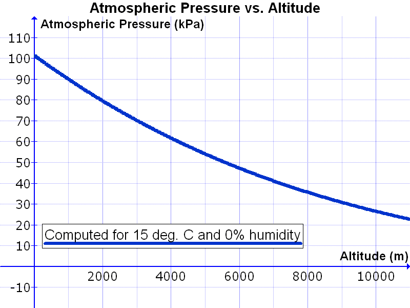 English: Graph of atmospheric pressure (in kPa) vs...
However we have yet to explain the intercept produced.
For an ideal gas P 1/V, thus creating a straight line graph passing through the origin proving no other parameters i.e. mass or temperature of gas are changed.
As a straight line graph is produced that does not pass through the origin we can say that the most likely cause of the non-zero pressure intercept came in the calibration of the pressure sensor. Before any readings were taken the pressure sensor had to be calibrated and an approximate value of atmospheric pressure was set, 100kPa. This was not a precise value, but we now are able to say the atmospheric pressure on that day was around 92kPa. If this adjustment were made to each of the pressure values recorded a straight line graph passing through the origin would have been obtained, proving pressure is inversely proportional to volume.
There are a few other sources of error in the experiment that also can be looked at. Firstly, the reading of the pressure on the digital pressure sensor would not have been completely precise. As it read to 0.1kPa we must assume all readings taken are only accurate to ñ.01kPa. However, the smallest pressure reading recorded was 32kPa, therefore an uncertainly of 0.1kPa would only have lead to a 0.3% uncertainty in the actual recorded value. As the pressure readings increased in size this percentage uncertainly would decrease further and is therefore negligible throughout the experiment.
Another source of error would have been the reading of the volume obtained, as this would not have been precise. As the reading of volume was read off using eye-sight a parallax error would have been produced. We can say that an uncertainty of ñ1cm3 could have been introduced into the values of volume recorded, therefore producing an maximum uncertainty of 5%. This is a far more substantial uncertainty and as it would be systematic it could have altered the position of the lines plotted on the two graphs.
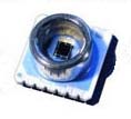 Digital air pressure sensor
 English: digital barometric pressure sensor BMP085...
 Atmospheric pressure and decompression
Boyles Law
i actually studied Boyles law and some of these things i wasnt aware of its intersting to see the things u didnt know about even after studying about it.
2 out of 2 people found this comment useful.