CHAPTER 20
DEMAND AND SUPPLY ELASTICITY
I. Price Elasticity of Demand
A. Concept of Price Elasticity
The responsiveness or sensitivity of quantity
demanded to a change in price.
B. General Formula for Price Elasticity
Percentage change in quantity demanded
Percentage change in price
C. Mid-Points Formula
E/demand =
D. Interpreting the Elasticity Coefficient
A coefficient higher than 1 is elastic
" " lower " 1 is inelastic
" " exactly 1 is unitary
A negative coefficient implies that a lower
price results is lower quantities sold.
E. Extreme Elasticities
Perfectly Elastic Perfectly Inelastic
Demand or Supply Demand or Supply
II. Total Revenue Test
If Demand is Elastic If Demand is Inelastic
P TR P TR
P TR P TR
III. What Determines Price Elasticity
A. The number and quality of substitute goods.
B. The proportion of income the purchase makes up.
C. The size of the expenditure.
D. The time available for adjustments.
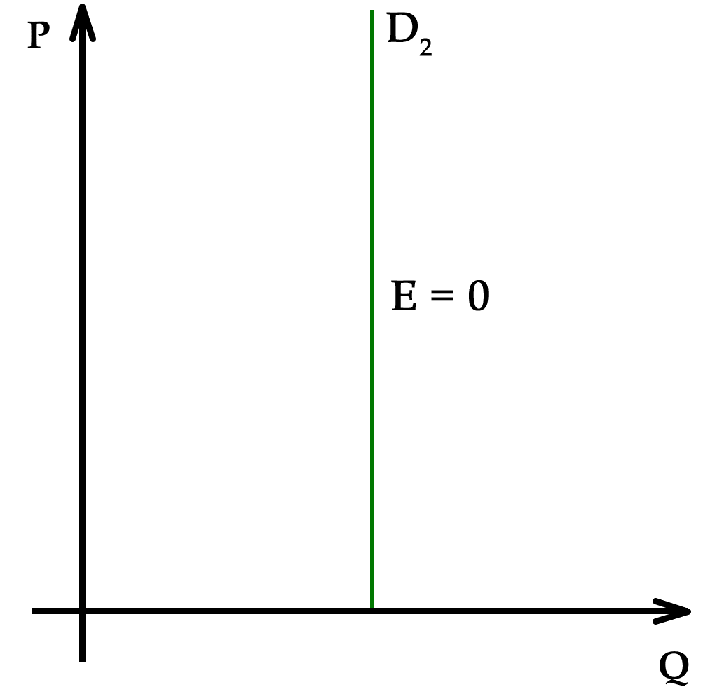 Perfectly inelastic demand
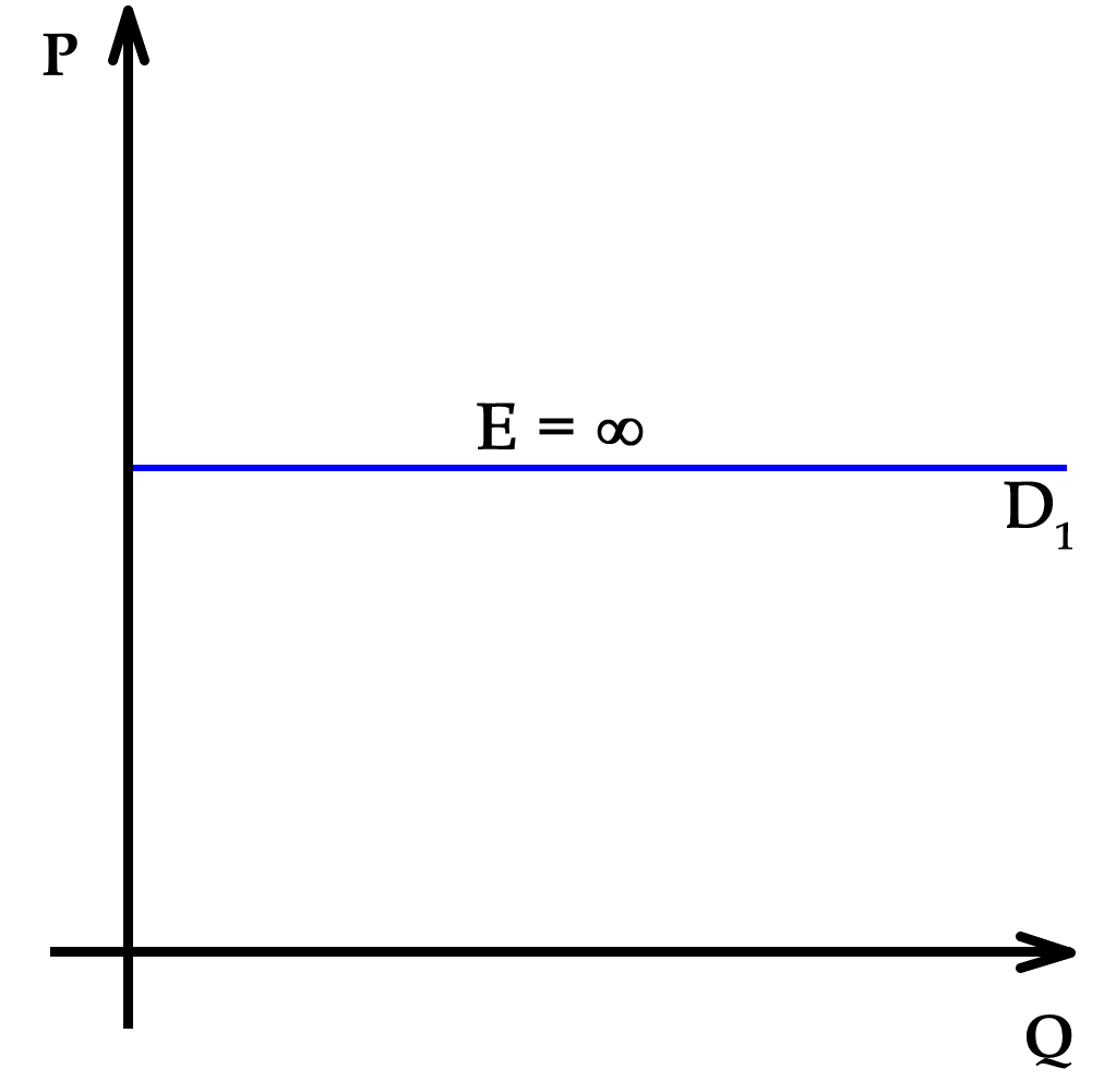 Perfectly elastic demand
 Graphical explanation of the total revenue test to...
E. Luxuries tend to be elastic.
F. Necessities tend to be inelastic.
G. Durable goods tend to be elastic. H. Promotion.
IV. Cross Elasticity of Demand
Shows whether two goods are substitutes or
complements.
Cross Elasticity Percentage Change in Q
Formula Percentage Change in P
If two goods are substitutes, the coefficient will be
positive.
If two goods are complements, the coefficient will be
negative.
V. Income Elasticity of Demand
Shows the responsiveness of certain goods to changes
in real consumer income.
Income Elasticity % Change in Q Demanded
Formula % Change in Real Income
Income-sensitive products have a coefficient higher
than 1.
The coefficient will vary according to income level.
VI. Elasticity of Supply
Shows the responsiveness of quantity supplied to a
change in price.
General Percentage Change in Q Supplied
Formula Percentage Change in Price
Determinants of Supply Elasticity
A. Short-Run Period (inelastic supply)
B. Long-Run Period (more elastic supply)
C. Market Period (short= inelastic; long= elastic)
VII. Applications of Price Elasticity of S and D
A. Wage bargaining (wage give-backs may save jobs if
the product is income-sensitive/ elastic)
B. Bumper crop in agriculture (will reduce the total
revenue of farmers, since products are inelastic.)
C. Automation (if the product is elastic, workers
displaced by automation, may be rehired)
D. Deregulation (works well on elastic goods)
E. Excise taxes, sin taxes (should be applied to
inelastic goods in order to enhance tax revenue)
CHAPTER 21
THE FINANCIAL ENVIRONMENT OF BUSINESS
I. The Legal Organization of Firms
A. Single Proprietorships (over 13 million, 74.3%)
Advantages:
1. Easy to organize
2. The owner is his own boss
3. All profits go to the owner
Disadvantages:
1. Unlimited liability
2. Limited financial resources
3. Owner is responsible for all decisions
B. Partnerships (1.7 million, 7.1%)
Advantages:
1. Easy to organize.
2. Easier to raise capital.
3. More specialization in management.
Disadvantages:
1. Unlimited liability
2. Each partner is responsible for the actions
of all other partners.
3. Division of authority leads to discord
4. The withdrawal of one partner ends the
business.
C. Corporations (over 3 million, 18.6%)
Definition: An artificial person, invisible,
intangible, and existing only in the eyes of the law.
Advantages:
1. Limited liability of stockholders.
2. The ability to raise capital by selling stock.
3. Larger size permits specialization, efficiency
4. Continuity of life ensured.
5. Separation of ownership and control.
Disadvantages:
1. Legally more complex.
2. Principal-agent problem.
3. Double taxation of corporate profits.
II. Methods of Corporate Financing
A. Share of Stock (ownership)
Legal claim to a share of the firm's future profits.
Common stock entails voting rights.
Preferred stock gives preferential treatment in the
payment of dividends. (no voting rights)
Stocks have no maturity dates.
Stockholders have a claim on the company's assets
only after all creditors had been paid off.
B. Bonds (corporate debt)
Interest must be paid on time.
Bondholders have no voice in management.
Bonds have a maturity date.
Claims of bondholders are satisfied before stock-
holders.
C. Secondary Market
Market for previously issued stocks and bonds.
D. The Stock Market
1. Random Walk Theory -future stock prices are
unpredictable.
2. Inside Information (illegal to use)
3. Price/ Earnings Ratio
Price of stock divided by earnings per share
4. Yield (%): Dividend per year divided by the
price of stock.
5. Dividend: dollars paid per share
E. Global Capital Markets
III. Problems in Corporate Governance
A. Separation of Ownership and Control
B. Asymmetric Information: Unequal sharing of
information.
C. Adverse Selection: The worst credit risks are the
ones likely to seek loans.
D. Moral Hazard: borrowers are likely to engage in
risky behavior resulting in default.
E. Incentive-Compatible Contract: pledging part of
corporate assets as collateral.
CHAPTER 22
COST AND OUTPUT DETERMINATION
I. Costs of Production
A. Explicit Costs (contractual costs)
Payments to outsiders for labor, materials, fuel,
transportation, rent, etc.
B. Implicit Costs
The cost of self-employed, self-owned resources,
such as the value of one's labor in its best alterna-
tive use.
C. Normal Rate of Return
The going rate to be paid to the investor for
employing his resource. (A cost of production)
D. Opportunity Cost of Capital
The income a resource would generate in its best
alternative use.
II. Profits
A. Normal Profit (Normal Rate of Return)
The minimum payment required to keep the
entrepreneur in business.
B. Economic/ Pure Profit (Not a cost of production)
Profits in excess or Normal Profit. (Total Reve-
nues minus Opportunity Cost of All Inputs)
C. Accounting Profit
Total Revenue minus Explicit Cost
D. Total Profit (Total Revenue minus Total Cost)
III. Types of Costs
TFC = Total Fixed Cost (overhead) It must be paid
even if output is zero. Examples: debt servicing,
depreciation, mortgage, property taxes, insurance.
TVC = Total Variable Cost. This cost changes with
output. Examples: labor, energy, raw materials.
TC = Total Cost (TFC + TVC)
MC = Marginal Cost. The increase in total cost
resulting from the production of an additional
unit of output. MC =
When Marginal Product is rising, MC is falling.
AFC = Average Fixed Cost AFC =
AVC = Average Variable Cost AVC =
ATC = Average Total Cost ATC =
or AFC + AVC
IV. Types of Products
TP = Total Product (output or Quantity Produced)
MP = Marginal Product. The increase in TP resulting
from the use of an addition unit of labor input.
The point where MP begins to fall is the Point
of Diminishing Returns.
AP = Average Product. Total Product divided by
Labor Input.
V. Types of Revenues
TR = Total Revenue (Output times Average Revenue)
MR = Marginal Revenue. The increase in TR upon
selling an additional unit of output. MR =
AR = Average Revenue. Total Revenue divided by
output sold. AR =
VII. Short vs. Long Run
A. Short Run Period. At least one factor of production,
usually capital, is fixed. Fixed costs exist only in
the short run.
B. Long Run. All costs are variable in the long run.
Plant size and all inputs can be varied.
VIII. Relationship between Average and Marginal
Costs The Marginal Cost curve always intersects the
ATC and AVC curves at their lowest points
IX. Long Run Cost Curves
A. Falling LR-ATC
B. Constant LR-ATC
C. Rising LR-ATC
D. Minimum Efficient Scale
The output range in which LR-ATC remains at
a minimum
E. Planning Horizon in the Long Run
CHAPTER 23
PERFECT COMPETITION
I. Characteristics
A. A large number of buyers and sellers.
B. Homogeneous/ standardized product
C. Free entry in/ exit from industry
D. Producers have no control over price.
E. Information is freely available to both buyers
and sellers
F. No non-price competition (No advertising)
G. No government intervention.
H. Example: agriculture
II. Demand Curve of the Perfectly Competitive
Producer
The D curve is perfectly elastic. Reason: each produ-
cer is too small to make an impact on industry supply.
Industry D curve is down-sloping.
The Average Revenue and Marginal Revenue Curves
are the same.
III. Profit Maximization in the Short Run
A. Total Revenue - Total Cost Approach
B. Marginal Revenue - Marginal Cost Approach
IV. The Short-Run Break-Even Point
The point where Average Total Cost = Price
V. Operating While Suffering Losses
Price is between Average Total Cost and AVC
VI. Short Run Shut-Down Price
The point where price drops below AVC
VII. Short Run Supply Curve of the Perfectly
Competitive Producer
That portion of the MC curve which rises above the
Average Variable Cost Curve.
VIII. Short Run Industry Supply Curve
The sum of quantities produced by all suppliers in
the short run.
IX. Long Run Industry Supply Curve
Reflects adjustments in the market supply after the
entry or exit of efficient/ inefficient producers.
X. Long Run Equilibrium
The output level at which
MR = MC = LRATC = SRATC
Marginal Cost Pricing = The opportunity cost of
production equals Marginal Cost. (There is no pure
profit, only normal profit)
CHAPTER 24.
MONOPOLY
I. Characteristics
A. A single producer/ seller
B. No close substitutes for the product.
C. Sole control over price (price-maker)
D. Sole control over market supply.
E. Blocked entry
F. Goodwill advertising
G. Government control
H. Examples: public utilities, Intel (?); US
Postal Service
II. Barriers to Entry
A. Economies of scale
B. Cost of capital
C. Patent rights
D. Cost of research
E. Exclusive franchises
F. Control over raw materials.
G. Economic and political muscle
H. Exclusive distributorships, fair trade pricing
I. Tariffs and other government protection
III. The Monopolist's Demand Curve
As volume produced increases, market price
falls. The falling price is the monopolist's
Average Revenue (AR = D) curve. Marginal
Revenue (MR) will be even more sharply down-
ward sloping:
Output AR (price) TR MR
1 $ 7 7 7
2 6 12 5
3 5 15 3
4 4 16 1
5 3 15 -1
6 2 12 -3
IV. Profit Maximization under Pure Monopoly
Profit is maximized at the point where Marginal
Revenue (MR) equals Marginal Cost (MC)
V. Pricing Behavior of Monopolists
A. The monopolist does not charge the highest
possible price. Objective: highest total profit.
B. Monopolists may suffer losses.
C. Monopolists prefer to produce in the elastic
portion of the demand curve which is approp-
riate for price cuts to maximize total revenue.
D. Limiting profits to discourage rivals.
VI. Price Discrimination
The product is sold at different prices to
different buyers. Prices are not justified by
cost differences.
Conditions for Price Discrimination
A. Downsloping Demand Curve
B. Separation of market/ segregation of buyers
can be achieved at a reasonable cost.
C. Buyers must have different elasticities of
demand.
D. The firm must be able to prevent the resale
of the product.
E. Examples: peak-time energy/ telephone use;
postal service, airlines, train service, theaters
VII. The Economic/ Social Cost of Monopolies
A. A lower quantity sold at a higher price.
B. Contributes to unequal income distribution.
C. Large profits enable more research and more
rapid technological growth.
D. Greater efficiency due to mass production.
E. The creation of giant multinational corpora-
tions transcending national boundaries.
CHAPTER 25.
MONOPOLISTIC COMPETITION
OLIGOPOLY
I. Monopolistic Competition
A. CHARACTERISTICS
1. A large number of producers/ sellers.
Small market share. Independence.
2. A highly competitive market.
3. Product differentiation.
4. Some limited control over price.
5. Advertising and other non-price
competition.
6. Brand allegiance.
7. Easy entry/ exit.
8. Examples: small grocery stores, clothing
stores, gas stations, restaurants.
B. PRICE AND OUTPUT DETERMINATION
1. The Demand curve and the Marginal
Revenue curve are mildly downsloping.
2. Profit maximization/ loss minimization
occurs where MR = MC
3. Short Run Equilibrium occurs where
ATC = Demand (AR) (Zero econ. profit)
4. Note that MR is below Price (AR) at the
Short Run Equilibrium.
C. MONOPOLISTIC VS. PERFECT
COMPETITION
1. Both earn zero economic profit in the
long run.
2. Under perfect comp. P = MC
Under monopolistic comp. P > MC
3. ATC is higher and output is lower
under monopolistic competition,
resulting in underallocation of resources
4. Economic Efficiency: P = MC = ATC
Correct Resource Allocation: P = MC
Most Efficient Technology: P = ATC
D. PROS AND CONS OF ADVERTISING
Pros
1. Adds 2% to the GDP
2. Promotes product differentiation and
competition.
3. Finances the media.
4. Stimulates product development.
5. Provides information about new products.
6. Promotes employment.
7. Diminishes monopoly power.
Cons
1. Competitive advertising is persuasive,
not informative.
2. Diverts resources from the economy.
3. Results in higher product prices.
4. Self-canceling in nature.
5. Inconvenient to the public.
6. It may contribute to monopoly power.
(High cost may be a barrier to entry)
7. Advertising may reduce efficiency.
II. Oligopoly
A. CHARACTERISTICS
1. A handful of producers/ sellers
2. Pricing interdependence
3. Heavy promotion/ nonprice competition
4. Difficult but sometimes easy entry
5. Anti-trust regulation
6. Collusion or price competition
7. Differentiated or standardized products
8. Examples: tobacco, car, tire, cereal,
camera, computer, steel industry
B. RESULT OF INTERDEPENDENCE
1. The reaction of rivals is unpredictable
2. The Demand and Marginal Revenue
curves are difficult to estimate
3. Prices tend to be inflexible (sticky)
4. Prices are changed in unison
C. OLIGOPOLY MERGERS
1. Horizontal merger (firms producing
similar products in the same industry)
2. Vertical merger (buying up one's supp-
liers or customers in the same industry)
3. Conglomerate merger (buying up unre-
lated companies in other industries)
D. MEASURING CONCENTRATION
Concentration Ratio: market share of the
top four companies in an industry
E. COLLUSIVE OLIGOPOLY
Due to price-fixing and limits on quantity,
it has the same effect as monopoly.
(see market demand curve for monopoly)
1. Cartels (illegal in the US)
Formal written agreement to fix prices and
limit output. OPEC.
2. Obstacles to collusion
-Demand and cost differences (MR = MC
points do not coincide with output allowed)
-Number of firms and their sizes
-Cheating (secret price concessions)
-Recession (excess capacity, declining profits)
-Legal obstacles (anti-trust action)
3. Price leadership (tacit collusion)
F. GAME THEORY
An analysis of alternative outcomes from
various interactive patterns of the participants
Cooperative game = players collude to improve
their position/ make themselves better off
Noncooperative game = no collusion
Zero sum game = gains offset losses
Negative-sum game = players as a group lose
Positive-sum game = players as a group gain
Example: prisoners' dilemma
G. KINKED DEMAND CURVE UNDER
NON-COLLUSIVE OLIGOPOLY
Rivals ignore a price increase but match a price
cut. This creates a break in the MR curve, and
causes a king (steeper decline) in the D curve:
H. ECONOMIC IMPACT OF OLIGOPOLY
1. Smaller quantity at a higher price (maybe)
2. Poor allocation of resources.
3. Income inequality
4. Technological advance
5. Influence on legislation/ government
CHAPTER 26.
REGULATION AND ANTI-TRUST POLICY
I. Types of Regulation
A. SOCIAL REGULATION
Deals with conditions under which goods and
services are produced. Main concern: the impact
of production on society and the physical charac-
teristics of goods. (Consumer Products Safety
Commission, Occupational Safety and Health
Administration, EPA, Equal Employment Oppor-
tunity Commission)
B. INDUSTRIAL REGULATION
Deals with the overall performance of selected
industries. Objective: to maintain competition; to
approve/ scrutinize mergers, etc. (FCC, FTC)
C. PRICE REGULATION
1. Cost of Service: no monopoly profits allowed.
2. Rate of Return: normal/ competitive profits
allowed.
II. Behavior of Regulated Industries
A. CREATIVE RESPONSE
Complying with the letter but not the spirit of the
law.
B. CAPTURE HYPOTHESIS
Regulated industries impose their will upon the
regulatory agencies.
C. SHARE THE GAINS, SHARE THE PAINS
Regulators must take into account the interest of
three groups: the legislators, the regulated indust-
ries, and the consumers.
III. Cost of Regulation
The total cost of government regulation is
estimated to exceed $600 billion annually, about
8% of the nation's income.
IV. Deregulation
A. Short Run Effects
1. Monopoly profits may disappear
2. Loss of employment and income
3. Level of service may decline
4. Some companies may go bankrupt
These negative effects may be offset in the long
run by lower prices due to increased competition.
B. Theory of Contestable Markets
Competitive conditions may exist even if there are
only a few producers in an industry. A market is
contestable if there is easy entry/ exit.
V. Federal Anti-Trust Laws
A. THE SHERMAN ACT OF 1890
No firm, state, or individual may conspire to
restrain trade or monopolize. (Poor enforcement)
B. THE CLAYTON ACT OF 1914
1. outlaws price discrimination
2. forbids tying contracts
3. prohibits the purchase of competitors' stocks
4. prohibits interlocking directorates
C. FEDERAL TRADE COMMISSION ACT (1914)
1. Public hearings to investigate unfair competi-
tion. "Cease and desist" orders.
2. Establishment of the FTC
3. Amended in 1938: the Wheeler-Lea Act
directed against deceptive advertising.
D. ROBINSON-PATMAN ACT (1936)
Directed against discriminatory pricing, discounts
or other concessions designed to lessen competit.
E. CELLER-KEFAUVER ACT (1950)
Eliminated a loophole under the Clayton Act:
firms could no longer purchase the physical
assets of competing firms, in addition to stocks.
VI. Exemptions from Antitrust Laws
Some exemptions include labor unions, public
utilities, professional baseball, hospitals, public
transit authorities, military suppliers
VII. Enforcement of Antitrust Laws
Market share test: a market share of 70% or
more constitutes monopoly as a rule of thumb,
but a smaller percentage may qualify based on
the existence of substitutes (tea/ coffee) and
geographic boundaries.
CHAPTER 27.
LABOR DEMAND AND SUPPLY
I. Reasons for Studying Labor Costs
A. They comprise a high percentage of total cost.
B. They ration labor to various industries.
C. They determine the combination of labor and other
resources to be used.
D. They determine personal income distribution, the
ratio between profits and wages, and the incomes
of various professions.
II. Marginal Physical Product of Labor
A. Demand for labor is derived from demand for the
product or service it produces.
B. Marginal Physical Product refers to the change in
output resulting from the use of an additional unit
labor.
C. The Marginal Physical Product declines because of
the Law of Increasing Marginal Costs.
III. Marginal Revenue Product of Labor
A. Marginal Revenue Product = The increase in total
revenue generated by an additional unit of labor
Marginal Physical Product x Marginal Revenue
(MRP = MPP times MR)
B. Marginal Factor Cost = The cost of employing and
additional unit of labor. Under a perfectly compe-
titive labor market, MFC equals the wage rate.
Labor Marginal Total
Input Output Phys. Prod. Price Revenue MRP MFC
1 10 10 3 30 30 12
2 18 8 3 54 24 12
3 24 6 3 72 18 12
4 28 4 3 84 12 = 12
5 30 2 3 90 6 12
Rule for resource employment: the point where
Marginal Revenue Product equals Marginal Resource
Cost
The Marginal Revenue Product Curve is the
Labor Demand Curve of the firm.
IV. What Determines the Elasticity of Labor Demand
A. The rate of decline in the Marginal Physical Prod.
(If MPP declines slowly, MRP also declines
slowly, and the Labor Demand Curve is elastic)
B. Elasticity of Product Demand. (If demand for the
product is elastic, Labor Demand is elastic, too)
C. The ease of resource substitutability. (The more
substitutes exist for the product, the greater the
elasticity of demand for labor)
D. Labor Cost-Total Cost Ratio. (The greater the
share of labor in total cost, the greater the elas-
ticity of demand for labor)
V. Wage Determination under Imperfect Competition
Under imperfect competition the product price falls
and wage rate increases with rising output. As a result,
MRP falls, and MFC increases: Wage
Labor Output MPP Price TR MRP Wage Cost MFC
1 10 10 3 30 30 4 4 4
2 18 8 2.75 49.5 19.5 6 12 8
3 24 6 2.50 60 10.5 7.5 22.5 10.5
4 28 4 2.25 63 3 10 40 17.5
5 30 2 2 60 -3 12 60 20
The equilibrium wage rate is determined by the point of
intersection between the MRP and the MFC curves. This
shows that the company will hire three units of labor at
a wage rate of $10.50, and output will be set at 24 units.
VI. What May Change the Demand for Labor?
A. Demand for the product labor produces.
B. Changes in productivity which may be due to
1. better technology
2. higher quality of labor or management
3. change in the combination of labor and capital
C. Market demand for labor = the sum total of each
firm's labor demand curve in the industry.
D. The type of competition that exists in the industry.
(Monopolists hire fewer workers than competitive
firms)
VII. Wage Issues
A. The real minimum wage is directly related to teen-
age unemployment.
B. Efficiency wage: a higher than competitive wage
rate which tends to ensure lower labor turnover
and higher labor productivity.
C. Insider-outsider theory: workers holding jobs at an
enterprise try to keep out any outsiders who might
be willing to work for less.
VIII. What Determines Labor Supply?
A. Wage rate changes in other industries.
B. Changes in working conditions.
C. Job flexibility and job sharing.
IX. The Optimum Combination of Resources
A. The Profit Maximizing Rule
1. Under Perfect Competition
MRP of Labor MRP of Capital
Price of Labor Price of Capital
2. Under Imperfect Competition
MPP of Labor MPP of Capital
MFC of Labor MFC of Capital
B. Least Cost Rule
The firm will hire resources up to the point where
the MPP of the last dollar spent is the same for
each resource:
MPP of Labor MPP of Capital
Price of Labor Price of Captial
(Cost per unit of service)
CHAPTER 28.
UNIONISM AND LABOR LAWS
I. Types of Unions
A. CRAFT UNIONS
They are composed of skilled craftsmen of given
trade or vocation.
They maximize their income by limiting member-
ship through
- examinations and occupational licensing
- initiation fees, long apprenticeship period
- legislation to require the use of union labor
- restriction on interstate movement
Examples: plumbers, electricians, carpenters
B. INDUSTRIAL UNIONS
They maximize power by including all workers of
an industry. They have a social/ economic agenda.
Objectives: political influence, power to workers,
social change, influencing government actions.
Examples: Teamsters, United Mine Worker, UAW
(Congress of Industrial Organizations -CIO)
II. Collective Bargaining
Negotiation between management and union
leaders to achieve a mutually acceptable labor
contract.
III. History of Unionism
A. REPRESSION PHASE (1790-1932)
1. Criminal conspiracy doctrine
2. Injunction - court order against strikes/ pickets
3. Blacklisting, discharge for union activity
4. Lockout - shutting down business for weeks
5. Hiring strikebreakers (scabs)
6. Yellow dog contract (promise not to join union)
7. Paternal/ company unions (run by management)
B. ENCOURAGEMENT PHASE (1932-1947)
1. Norris-Laugardia Act (1932)
Eliminated injunctions/ yellow dog contracts
2. Wagner Act (1935) National Labor Relations
Act. Established the NLRB
Gave workers the right to strike without penalty
and to engage in collective bargaining.
C. INTERVENTION PHASE (1947- Present)
1. Taft-Hartley Act (1947) Key provisions:
a. Eliminated unfair union practices:
- coercion to join
- jurisdictional strikes (fight over which union
should perform a job)
- secondary boycotts (refusal to buy the products
of competing unions)
- sympathy strikes (in support of other unions)
- large initiation fees
- featherbedding
b. Regulated union contracts:
- required financial reports to the NLRB
- regulated political contributions
- required non-communist affidavits
c. Regulated contract content
- outlawed closed shop
- check-off had to be authorized by workers
- separated welfare and pension funds
- introduced reopening clauses
- introduced the 80-day cooling-off period
2. Landrum-Griffin Act (1959)
Regulated the election of union officers.
IV. Business Unionism
The American Federation of Labor (AFL) created
in 1886. First president: Samuel Gompers. Principles:
A. Rejection of socialism
B. Objectives limited to better pay, shorter hours,
better working conditions, fringe benefits
C. Political neutrality - non-interference by gov't
D. Autonomy of craft unions within the AFL
V. Government Regulation
A. Right-to-Work Laws - make it illegal to require
union membership as a condition of employment
B. Union Shop - requires a promise from new workers
to join the union within 30 days (illegal in states
which have right-to-work laws)
VI. Union Goals
A. Setting wage above the market rate.
B. Providing employment for all members
C. Restricting labor supply
D. Increasing worker productivity
E. Increasing demand for union-made goods
VII. Benefits of Labor Unions
A. Promoting better working conditions; social
efficiency
B. Reduction of wage inequality
C. Reduction of monopoly profits
D. Giving political voice to workers. Influence on
legislation
E. Reduction of workplace friction through orderly
arbitration and grievance procedures
VIII. Monopsony Model
A single buyer for labor. Example: professional and
college sports.
Monopsony Model Bilateral Monopoly Model
IX. Bilateral Monopoly Model
A national labor union facing a monopsonist.
Example: The United Mine Workers against a
mining company which owns virtually all the
jobs in a town.
CHAPTER 29.
RENT, INTEREST, PROFIT
I. Rent
A. ECONOMIC RENT
Payment received for a resource over and above its
opportunity cost.
Additional land rent has no incentive function to
generate more land because the supply of land is
fixed (perfectly inelastic).
B. Function of economic rent: it allocates resources
their highest-valued use.
C. Economic rent to labor: income earned over and
above labor's second best alternative use.
Examples: movie stars, rock stars, sports heroes
II. Interest
A. Definition: price paid for the use of someone else's
money. (Borrower is actually buying time)
B. What determines the interest rate:
1. Length of loan.
2. Risk.
3. Size/ type of loan.
4. Handling charges.
5. Market imperfections.
6. Supply and demand of loanable funds
C. Case study: Rent-to-own stores
D. Equilibrium Interest Rate:
E. Nominal vs. Real Rate of Interest
Nominal: stated interest rate in current dollars
Real: Nominal minus Anticipated Inflation
F. Allocative Role of Interest
Interest allocates loanable funds to their most
profitable uses.
G. Interest and Present/ Future Value
Present Value of Future Dollars: An amount
to be received in the future has a smaller value
today. (see table on p. 659)
An amount paid out today has a greater value
in the future.
III. Profits
A. Economic Profit
Total Revenue less Explicit + Implicit Costs
B. Accounting Profit
Total Revenue less Explicit Costs
C. Sources of Economic Profit
1. restricted entry of rivals
2. innovation, new ideas
3. risk taking (payment for uninsurable risks)
4. providing a service to society
5. giving employment opportunities to others
D. Functions of Economic Profit
1. profit encourages innovation/ investment
2. profit shows the direction the economy should
take
3. profit ensures the efficient allocation of
economic resources
CHAPTER 30.
INCOME, POVERTY, AND HEALTH CARE
I. Income
A. THE LORENZ CURVE
Shows the inequality in income distribution among
the five quintiles of the economy.
The 45-degree line represents perfect income
equality. The field between the curve and the 45-
degree line shows the inequality gap.
B. CRITICISMS OF THE LORENZ CURVE
1. it does not show income received in kind
2. it does not show differences in the size of
households
3. it does not account for the age differences
of families (older people tend to earn more)
4. it reflects income before taxes
5. it excludes all unreported income
C. CAUSES OF INCOME INEQUALITY
1. ability differences
2. education/ skill level
3. level of ambition
4. job tastes
5. willingness to take risks
6. property ownership
7. market power (legislation, inside info.)
8. luck, connections, discrimination
D. DISTRIBUTION OF WEALTH
Richest 1% owns 36% of all assets
Next 9% owns 31% of all assets
Richest 10% owns 67% of all assets
Remaining 90% holds 33% of all assets
E. DETERMINANTS OF INCOME DIFFERENCES
1. Age Earnings Cycle
The average person's income peaks at age 50
Intergenerational Mobility: income rises from
one year to the next.
2. Intragenerational Mobility
Successive generations earn more than their
forefathers
3. Marginal Productivity
With increasing skill and experience people
become more productive.
4. Investment in Human Capital
Treating education/ retraining as an investment
F. EGALITARIANISM vs. EFFICIENCY
Equality in income distribution would maximize
consumer satisfaction from the national income
but it would remove the incentive to work
Comparable worth doctrine: women should earn
the same wages as men if they hold the same job
and have the same skills as men.
II. Poverty
A. Poverty in the US and the world
The number of Americans officially below the
poverty line is about 37 million.
In 1996 the official poverty level for an urban
family of four was $16,000.
According to the UN, 1,300 million people live
in poverty worldwide.
B. Income Maintenance Programs
1. Social Security (OASDI = Old Age, Survivors'
and Disability Insurance) 90% of working men
are covered by Social Security in the US. At this
time about 50 million people receive benefits
averaging $713 per month.
2. Supplemental Security Income (SSI), Aid to
Families with Dependent Children (AFDC)
3. Food Stamps. The program has more than 28
million recipients at an annual cost of 30 billion.
4. Earned Income Tax Credit (EITC)
Provides benefits up to $2,528 for those with
incomes between $8,425 and $11,000. In Missi-
ssippi and DC nearly half the families are
eligible. Nationwide eligibility: 20%
III. Health Care
A. Health Care Spending
In 1965 health care costs were 6% of natl. income
In 2000 health care costs will be 15 % " "
B. Reason for High Costs
1. The top 5% of health care users incur 50% of
all costs.
2. The population is living longer. The top 5%
is made up of people 70 and older.
In 1996 12% of the population was over 65
In 2035 22% " " " will be over 65
3. Costly new technologies
4. Third-party financing tends to increase demand
for health care
5. Moral hazard. Role of the deductible.
6. Abuses by health care providers.
C. Dealing with Health Care Costs
1. National Health Insurance
Would the healthy subsidize the chronically ill?
2. Medical Savings Accounts
Tax exempt employee savings. It would relieve
employers from providing zero-deductible health
care services.
3. Employee could apply unused MSA's toward a
supplementary retirement plan.
4. Moral hazard (seeking medical care when unne-
cessary) would be reduced.
IV. Discussion on Welfare Reform
A. Do high welfare benefits reduce the incentive to
work?
B. Are government sponsored job training programs
effective in reducing dependence on welfare?
C. The "leaky bucket" theory of welfare.
D. Pro's and con's of the negative income tax.
Objectives:
1. to get people out of poverty
2. to provide incentives to work
3. costs should be reasonable
No plan can meet all goals some of which are
mutually exclusive.
E. Relationship between income distribution and
the overall efficiency of the economy.
F. What is net worth? What is the difference between
income and wealth?
G. How can we reform federal Medicare spending?
CHAPTER 31.
ENVIRONMENTAL ECONOMICS
I. Private vs. Social Costs
A. Private Costs (Internal Costs)
They are paid by the individuals/ firms that incur
them.
B. Social Costs
The sum total of private (internal) and external
costs imposed upon society.
II. Externalities
A. Definition
Externalities develop when private costs diverge
from social costs.
B. How to Correct for Externalities?
1. require the installation of pollution abatement
equipment
2. cut pollution-causing activity
3. pay an ongoing fee for pollutants emitted
4. create a market for pollution rights
5. apply punitive taxes against polluters
6. force polluters to pay for the cleanup
C. "Optimal" Quantity of Pollution
Point of intersection between the marginal cost and
marginal benefit of pollution abatement.
D. Problems of Assigning Responsibility for Pollution
1. Determining property rights
Private Property: exclusive ownership rights
Common Property: air, water, etc. owned by all,
therefore by none
2. Responsibility for pollution is easily assigned
when private property rights are involved. The
same is not true for common property.
3. Transaction Costs: costs associated with reach-
ing and enforcing agreements (pertaining to
pollution)
III. Recycling
A. Benefits and costs.
B. Is the world running out of scarce resources?
CHAPTER 32.
PUBLIC CHOICE:
THE ECONOMICS OF INTEREST GROUPS
I. Collective Decision Making
The manner in which voters, politicians, and interest
groups influence public choice. The Theory of Public
Choice is simply the study of collective decision-
making.
II. Differences between Private and Public Choice
A. Public goods are provided at no cost to the user
B. The gov't can use force to achieve its objectives
C. The political system is run by majority rule 51:49%
D. The private economy is run by proportional rule.
(Dollar votes express the intensity of a want)
III. The Iron Triangle
It is an alliance of bureaucrats, interest groups
(lobbies), and congressional committees which parti-
cipate in making public choices.
IV. Interest Groups
A. Distributional Coalitions
Special interests, unions, and professional organi-
zations representing their members. Their interest
is concentrated while the public interest is diffused.
B. Logrolling
Elected representatives exchange political favors
at public expense.
V. The Role of Bureaucrats and Politicians
A. Rational Ignorance
Voters prefer to delegate their vote to elected repre-
sentatives in order to minimize the time invested in
making public choices.
B. Paradox of Voting
People are unable to rank public choices that might
benefit them.
C. Median Voter Model
Politicians tend to gravitate toward the center to
ensure mass-appeal.
D. Nonselectivity
No single bundle of public goods fits the needs of
any single voter perfectly.
VI. Political Rent-Seeking
The use of private resources in an attempt to get
government benefits for special interest groups.
VII. The Farm Problem
A. History of the Farm Problem
1. 1900-1915 was the golden age of US agricult.
2. By 1960 farm income fell to 50% of non-farm
income
3. The proportion of US population living on farms
dropped from 43.8% (1880) to 1.8% today
B. Causes of the Farm Problem
1. Long-Run Causes
a. inelastic demand for farm products
b. rapid improvements in technology
c. lagging demand for farm products
d. immobility of resources
2. Short-Run Causes
a. fluctuations in output due to weather
b. fluctuations in domestic/ foreign demand
c. high fixed cost of equipment
C. Public Policy toward Farmers
1. The policy has been based upon the assumption
that the farm is the last remaining bastion of
perfect competition.
2. Price Supports (minimum guaranteed price) The
government buys up the surplus.
3. Price Subsidies (a price below equilibrium with
payments made to farmers as an offset)
4. Target Price (The use of deficiency payments to
guarantee the farmer the targeted price)
5. Parity Ratio
Prices received divided by Prices paid
The adjustment of farm income to increases in
the cost of living & operating a farm.
6. Surplus Controls
a. restricting supply (acreage rotation/ reserve)
b. new uses for farm products
c. giveaways (food stamps, school lunch, aid)
CHAPTER 33.
WORLD TRADE
I. The Importance of World Trade
A. Volume
Since 1950 the world's GDP has increased 6-fold
while the volume of trade has gone up 13-fold.
B. Dependence on Trade
In 1950 imports in the US added 4% to annual
income, today they add 12%. In other countries
import dependence is much greater.
II. Beneficial Effects of World Trade
A. Gains from trade increase living standards
B. Trade allows increasing use of worldwide speci-
alization (taking advantage of comparative
advantage)
C. Trade leads to a better allocation of the world's
resources
D. Product and resource prices move toward equality
III. Obstacles to Trade
A. Politics (embargo, tariffs, quotas)
B. Currency/ exchange rate differences
C. Pressures to achieve a trade surplus
D. Negative Terms of Trade (ToT= Export Prices
divided by Import Prices)
IV. Comparative Advantage
A. The ability to produce a good at a lower opportu-
nity cost than one's trading partners
B. Gains from trade through specialization
V. Exports and Imports
A. In the long run, imports are paid for by exports
B. Restrictions imposed on imports will eventually
result in lower exports
C. Dumping (selling below domestic price or pro-
duction cost)
VI. Arguments against Free Trade
A. Military self-sufficiency
B. Protection of domestic employm./ living standards
C. Infant industry argument
D. Diversification for stability
VII. Quotas
Limitation on the quantity to be imported
VIII. Tariffs
Import duties imposed on foreign goods
IX. GATT and the WTO
GATT (General Agreement on Tariffs and Trade),
established in 1947, and the WTO (World Trade
Organization), established in 1995 aim to reduce
tariffs and trade barriers worldwide.
CHAPTER 34
EXCHANGE RATES & BALANCE OF
PAYMENTS
I. Balance of Trade vs. Balance of Payments
A. Balance of Trade shows the difference between
exports and imports.
B. Balance of Payments is a summary of all economic
transactions with the rest of the world. It includes
trade, transportation, tourism, military spending,
interest and dividend income, sale of assets, sale
of gold, and currency exchange
II. Current Account Transactions
A. Merchandise Trade $ - 161 bill.
B. Export and Import of Services + 68 "
C. Unilateral Transfers - 30 "
Total: - 191 + 68 = - 123 bill
III. Capital Account
A. US Capital Going Abroad - 314.8
B. Foreign Capital Coming In + 431.5
C. Official Transactions + 6.3
+ 123 Bal: 0
IV. Official Reserve Account Transactions
A. Foreign Currency Exchange
B. Sale of Gold
C. Special Drawing Rights with the IMF
D. Reserve Status at the IMF
E. Holdings of the US Treasury
V. What Affects the Balance of Payments
A. Relative Rate of Inflation (higher inflation worsens
the balance of payments)
B. Political Stability (stability improves the balance)
VI. Exchange Rates
A. Flexible/ Floating Exchange Rate
The rate is determined by the supply and demand
of currencies.
B. Appreciation of a Currency
An increase in the value due to increasing demand
for the nation's goods in world trade
Curve: An increase in demand for German-made
goods means higher demand for German Marks,
and a higher dollar cost of the DM:
C. What Determines Exchange Rates
1. Interest Rates (Higher rate=stronger currency)
2. Productivity (Higher prod.=stronger currency)
3. Changes in Product Preferences
4. Economic/ Political Stability
5. Relative Income Changes
VII. The Gold Standard and the IMF
A. Pegged/ Fixed Exchange Rates
They were based upon the gold standard. From
1933 to 1971 the $ was pegged at $35/ oz of gold
B. The Bretton Woods System (1945)
Established the IMF to help nations deal with their
balance of payments problems. Nations had to
intervene to keep the value of their currencies
within 1% of declared par value.
C. Special Drawing Rights (SDR's) (1967)
The IMF allocates SDR's to member nations based
upon a quota system
D. Removal of the Dollar from the Gold Standard
After Dec. 18, 1971 the $ was no longer exchange-
able for gold.
E. Dirty/ Managed Float of the $ (1973)
Exchange rates are determined by the supply and
demand of currencies but central banks may inter-
vene to "support" a currency in order to imporve
their trade position.
CHAPTER 19
CONSUMER CHOICE
I. UTILITY THEORY
A. Utility = the want-satisfying power of a good or
service
B. Marginal Utility = The increase in total utility upon
the consumption of an additional good or service
C. Total Utility = Satisfaction derived from the con-
sumption of all units of a good or service
D. The Law of Diminishing Marginal Utility = The
more units of a good we consume, the less our
additional satisfaction
Example:
Quantity of Big Macs Marginal Total
Consumed Utility Utility
1 10 10
2 4 14
3 - 4 10
(Total Utility reaches its peak at the point where
Marginal Utility is zero)
E. Optimization of Consumer Satisfaction
The consumer's income should be allocated so that
the last dollar spent on each product purchased
should yield the same marginal utility:
Marginal Utility of A Marginal Utility of B
Price of A Price of B
Example:
Quant. A Price MU of MU/ P Quant. Price MU of MU/P
of A of A A of A of B of B B of B
1 $ 4 20 5 1 $ 3 12 4
2 4 8 2 2 3 9 3
3 4 4 1 3 3 3 1
The consumer should purchase three units of each product
in order to maximize satisfaction from a budget of $ 21.
The consumer will always buy that product first which
yields the highest MU per dollar.
II. Assumptions about Consumer Behavior
A. The consumer is rational in making choices
B. The consumer is fully aware of the products features
and the value of each feature to him
C. The consumer's budget is limited (budget restraint)
D. Prices ration the goods available (budget line)
E. Income Effect = A decline in the price of a product
means an indirect increase in real income.
F. Substitution Effect = If the price of a good falls, con-
sumers will buy more of it, and less of its substitutes
whose prices are unchanged.
III. Budget Line = Shows various combinations of two
products which can be purchased on a given income
IV. Indifference Curve = Shows all combinations of
products A and B which yield the same level of total
satisfaction to the consumer
V. Indifference Map = A series of indifference curves, each
showing a different level of total utility
VI. Consumer Optimum = The point where the highest
indifference curve is tangent to the budget line.
VII. Income-Consumption Curve = The line connecting
points of consumer optimum as income increases
VIII. Price-Consumption Curve = The line connecting
points of consumer optimum as the price of a good
changes