⢠The data:We uses data from the Swiss health survey (SOMIPOPS) from 1982 thatis merged with tax assessment data (SEVS, Schweizerische EinkommensundVermèogensstichprobe). The sample contains 1761 individuals of Swissnationality. The Stata file sevs.dta contains the following variablesLMS labour market status (1 = employed, 0 = not employed)HRS working hours per weekWPH gross wage per hourNWI net non-wage incomeSEX gender (1 = woman)AGE ageHI health index (increasing with physical health)EDU education in years of schoolingEXP presumed work experience (age - education - 7)JO labour market situation (no. job offers/no. unemployed, cantonal)MAR marital status (1 = married, 0 = single, widowed or divorced)KT number of childrenK02 number of children between 0-2 yearsK34 number of children between 3-4 yearsK512 number of children between 5-12 yearsK1319 number of children between 13-19 yearsâ¢The AimThis project sets deals with non-linear functional form in the linear regressionmodel. While this topic is trivial in econometric theory. Application of great practical importance and a frequent source of mistakes.
 From http://hypernews.ngdc.noaa.gov
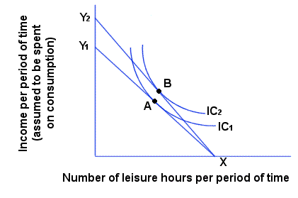 Effects of a wage increase
 The Stata Center houses CSAIL, LIDS, and the Depar...
⢠The TaskThis application deals mainly with hypotheses from the human capital theory.
.
a)Compare the earnings of men and women.
In order to compare the earnings of men and woman we have chosen the variable WPH - gross wage per hour - as the measure of earnings. If we look at the following Stata output:It turns out that, on average, men seem to have higher earnings than women.
Is this difference statistically significant? In order to answer this question we will perform a t-test that compares the means of two independent samples .
The Stata output is given by:The null hypothesis says that the difference of the means of the two samples is equal to zero. The resulting statistic is t = 11.8809 to which is associated a p-value of Pr(|T| > |t|) = 0.0000. So, with a 95% confidence level we can state that there's enough statistical significance to reject the null hypothesis that says that both samples have the same mean. In other words, we can infer that with a 95% confidence level there's enough statistical significance to say that on average men have higher earnings than woman.
b)Estimate the Mincer equation for all employed workers: log(wphi) = _0 + _1edui + _2expi + _3exp2i+ ui (1)The estimation of the Mincer equation is given by:c)Interpret _1. Calculate the marginal effect of education on wage.
measures the proportional or relative change in WPH (gross wage per hour) for a given absolute change in EDU (education in years of schooling). We can show it mathematically, as follows:In this specific regression =0.0774464, so wages increase by 7.74% for every additional year in education.
The marginal effect of education on wage is given by:=d)Test whether education has a significant effect on wage.
According to the Stata output from b) it follows that the coefficient relative to education is statistically significant with 95% of confidence level as the p-value = 0.00%. So it seems that education has a significant effect on wage.
e)Sketch the relationship between wage and work experience in a graph. Discuss the marginal effect of experience. Is there an optimal duration of experience?The graph that shows the relationship between wage and work experience is given by:If we look at the coefficients for the regression estimated in b) we conclude that the slope coefficient for experience is positive but the coefficient of the experience-squared variable is negative. Work experience seems to have a positive impact on wages, but this impact increases at a diminishing rate.
The optimal duration of experience is given at the point where:0For our estimated modelf)Test whether work experience has a significant effect on wage.
According to the Stata output from b) it follows that the coefficients relative to experience are both statistically significant with 95% of confidence level as their p-value = 0.00%. So it seems that experience has a significant effect on wage.
g)Introduce work experience as a spline function with 5-year intervals instead of the polynomial. Scetch the relationship. Test whether there is a negative effect of experience towards the end of the working live.
mkspline exp_1 5 exp_2 10 exp_3 15 exp_4 20 exp_5 25 exp_6 30 exp_7 35 exp_8 40 exp_9 45 exp_10 50 exp_11 =expregress lwph edu exp_1 exp_2 exp_3 exp_4 exp_5 exp_6 exp_7 exp_8 exp_9 exp_10 exp_11The first 15 years of work experience are relevant for the wage you can get. After the those years of experience, the wage does not depend anymore on the years of work experience.
For testing we can use a F-test, and we can see that between 30 and 50 years of experience this variable is not significant anymore, so this is consitent with the graph we use before in e), the relationship between wage and years of work experience is XXXtest exp_1 exp_2 exp_3 exp_4 exp_5test exp_6 exp_7 exp_8 exp_9 exp_10 exp_11h) Add a dummy variable to equation (1) to test whether there is a difference in earnings between men and women. Is the difference significant and substantial?If I include the dummy variable SEX (0=man, 1=woman) to my estimated model I get the following results:The log wage differential between man and woman is given by the coefficient of sex, which is estimated as being equal to -0.02845566. So, on average woman earn less 2.84% than man ceteris paribus. Given that the t-statistic for the estimated coefficient of sex is very high (in absolute terms) and its p-value is essentially zero, it can be inferred that there exists indeed a difference in earnings between men and women.
i)Interact all variables in equation (1) with the dummy variable for gender and add these new variables to the estimation: log(wphi) = _0 + _1edui + _2expi + _3exp2i+ _4sexi + _5edui ⢠sexi + _6expi ⢠sexi + _7exp2i⢠sexi + ui(2) Explain the meaning of the new parameters. What do the p-values in the Stata output test?The results of this new estimation are given by:The coefficient on sex is no longer statistically significant (t=-0.04) at conventional levels. I will explain why this is the case in answer k). The coefficient on "edusex" measures the difference in the return to education between men and women ceteris paribus but it is not statistically significant (t=0.44) at conventional levels. So we should infer that there is not statistical significance on the difference in the return to education between men and women. The coefficient on "expsex" measures the difference in the return to work experience between men and women ceteris paribus and it is statistically significant. The coefficient on "exp2sex" measures the difference on EXP^2 between men and women ceteris paribus. What do the p-values in the Stata output test?j)Is there a difference between the wage equation of men and women?We should compute an F-test with the following null hypothesis to infer if there's a difference between the wage equation of men and women:And the F-test is given by:Where q is the number of variables excluded in the restricted model, n is the number of observations, k is the number of explanatory variables including the intercept, SSRr is the residual sum of squares of the restricted model and SSRur is the residual sum of squares of the unrestricted model. We can take all the information from the Stata outputs, or simply perform the test in Stata:It comes that my F-statistic is given by 52.52 (as we can see in the stata output). The critical value (c) of a F-distribution with 5% of significance, numerator df of 4 and denominator df of 1218 is 2.21. My F-test is 52.52 >2.21, so we reject the null hypothesis and thus we can infer that jointly the coefficients for "sex", "edusex", "expsex" and "exp2sex" are statistically significant, which is translated into a difference between the wage equation of men and women.
k)Do the data reveal discrimation of women on the labour market?Although the coefficient on sex was not statistically significant in model i) we would be making a serious error to conclude that there is no significant evidence of lower pay for women (ceteris paribus). Since we have added the interaction terms to the equation, the coefficient on sex is now estimated much less precisely than in equation h): the standard-error has increased by more than six-fold (0.1234/0.0223). The reason for this is that "sex" and the interaction terms are highly correlated. In this sense, we should look at the equation in h) and conclude that there is indeed discrimination of women on the labour market as according to the coefficient on "sex", on average woman earn less 2.84% than man ceteris paribusl)Generate two new dummy variables MAN and WOMAN. Estimate the following equation log(wphi) = _0mani + _1edui ⢠mani + _2expi ⢠mani + _3exp2i⢠mani + _4womani + _5edui ⢠womani + _6expi ⢠womani + _7exp2i womani + ui (3) Explain the difference between (2) and (3). Test j) in equation (3).
In order not to have the so-called dummy variable trap we had to exclude the "overall" intercept. If we compare equation in i) with the one in l) we can infer that the first 4 coefficients are the same on both equations, which makes sense as we do not to have the dummy "man" in equation i) but we still have a dummy for sex. The differences between the two equations arise for all the explanatory variables which include (or interact) with "woman", as a new intercept=1.836534 is now presented in equation l). Note that this intercept is actually the sum of the overall intercept and the coefficient of sex in equation i) (1.841936+(-0.0054021)=1.836534). The same rationale is extended to the following coefficients, in the following way:m)Estimate (1) for men and women seperately. Spot the difference to (3) and discuss the different assumptions of the econometric models behind the estimated equations.
The regression for man is:The regression for woman:Separating equation (3) in two diferrentiated equations one for man and the other for women, we get the same coefficients for all variables as we can see above, but each one of them with a lower standard error. This means that the sepparated model is better specificated as the joint one (more precise).
Bibliography:http://www.springerlink.com/content/n1128j40w4365082/http://www.ncbi.nlm.nih.gov/pubmed/6229936
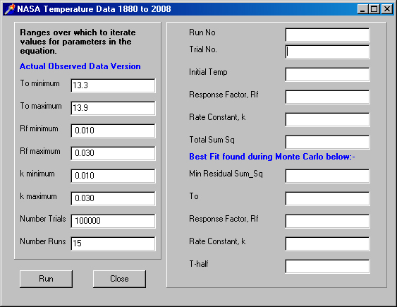 User interface for the simple Monte Carlo program ...
 MIT Stata Center
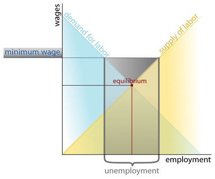 Wage labour