The expections-augmented Phillips curve Part ii 1. P = Pe + g (y "" y*) 2. R = a1 . y "" a2 . (m "" p) 3. r = R - Pe 4. y = b0 "" b1 . r 5. p = Lp + P Equation 1 is derived directly from the essence of the expectations-augmented Phillips curve. It states that actual inflation is equal to expected inflation when the unemployment rate is at the natural level. In other words, the unemployment rate differs from the natural rate when expected inflation does not match actual inflation. Unemployment is then substituted with output, y, and we end at equation 1. (See further explanation below). The parameter g determines how much a difference between output and potential output affects the inflation rate.
In the model, y is the log of GDP. This makes sense, because we are normally interested in percentage increases in GDP.
 English: Gross domestic product growth from 2007 t...
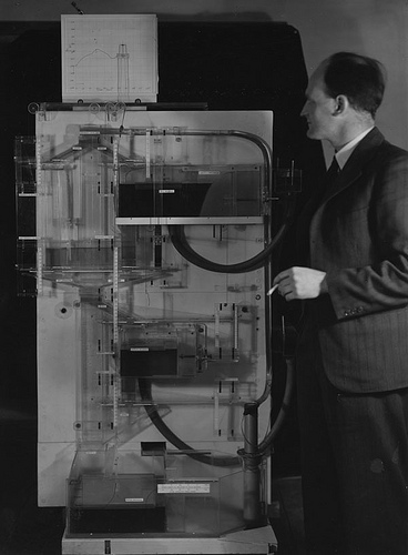 Professor A.W.H (Bill) Phillips with Phillips Mach...
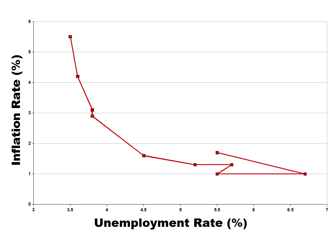 English: Relationship between the inflation rate a...
Using the log form means that a steady growth gives a linear function, whereas without the log form we would have to use an exponential functional form.
Equation 2, where R is the nominal interest rate, m is the log of the money stock and p is the log of the price level, states that the nominal interest rate is a function of GDP and the growth of the money stock and the price level. The first part of the equation (a1.y) means that when GDP increases this tends to push up R by the factor a1. The term (m - p) is the stock of real money balances. If prices are growing at a higher rate than the money stock, the stock of real money balances will decrease, and thus the nominal interest rate will increase. Equally, when the stock of money is growing...