Modeling to Produce music Juan Manuel Agudo Carrizo (UE2526361)
Digital Signal Processing Design Project
1. Digital Waveguide Modeling
For my project I have decided to model an acoustic guitar. Following the steps of : " Smith, Julius O. Digital Waveguide Modeling of Musical Instruments http://www-ccrma.stanford.edu/~jos/waveguide/".
The computer works in a discrete way, not in a continuous one, that means that it works with numbers, that we keep in vectors.
To make sounds we need a signal that in this case is a vector with a lot of numbers, that vector must contain the sound.
The sound is a vibration, a wave that we see in a sinusoidal way.
In the vector we keep the values of the signal. An analogy to understand this matter would be to visualize it this way: A string that is moving itself, vibrating, and in a certain moment we take a picture of it. When the string is not moving we say it has a zero value, while it is moving from left to right it is getting values, the ones we measure in the middle of the string from the point where it is quite. It biggest elongation will be 1 (to the right) and -1 (to the left):
As the movement is a vibration, I have to keep these values each certain time interval, it would be like taking pictures of my wave each second, now is when the concept of "sample frequency" receives a meaning.
The sample frequency "fs" is the quantity of samples (pictures in my analogy) that are taken in one second.
Now, we model the vibration of a string using a digital waveguide. "Two delay lines represent two travelling waves moving in opposite directions. By summing the values at a certain location along the delay lines at every time step, we obtain a waveform. This waveform is the sound heard with the pickup point placed at that relative location. The delay elements are initialized with a shape corresponding to the initial displacement of the string. For simplicity a triangular wave is used even though in reality the initial displacement of a plucked string will not be shaped exactly like a triangle. Simply using two delay lines in this fashion would require arbitrarily long delay lines depending on the length of the desired output. By feeding the delay lines into each other a system can be created that can run for an arbitrary amount of time using fixed size delay elements.
Digital waveguide with initial conditions of delay lines set to triangular waves.
In modeling a guitar it is important to note that the ends of the string are rigidly terminated, so the waves reflect at either end of the string. This effect can be modelled by negating each sample after it reaches the end of a delay line, before feeding it into the next delay line, as shown in Figure 1. Finally, we must add an attenuation factor. Without the attenuation factor, the model described up until now results in ideal string vibration that never decays. In the real world, due to friction and air resistance, the amplitude of the string vibrations decay over time, so it is important to model this effect in the digital waveguide. To attenuate the output we simply add a damping factor at the ends of the delay lines so that the values are damped before being fed into the other delay line.
Order N digital waveguide with rigid terminations corresponding
to the nut and bridge of a guitar
The length of the delay lines controls the frequency of oscillation, and consequently the pitch of the output signal. This corresponds to fretting a string on a guitar. Fretting a string limits the vibration to a certain length of the string. This changes the wavelength of the travelling waves, which in turn changes the pitch of the sound. Due to the looping nature of waveguide and the lack of additional input the output at every period is the same except attenuated slightly. Therefore the overall output will be periodic with a period depending to the length of the delay line. Therefore, if the desired frequency of the output is f and the sampling frequency is fs we set each delay line length to N/2 where N = fs/f.
The sound synthesized by this model sounds very artificial. It does nothing to account for the timbre of the instrument, and modeling the string pluck as a triangle wave is not very accurate. In addition, it does not take into account the fact that a real string vibrates in both the horizontal and vertical planes and interacts with the other strings on the guitar. Despite this, it is important to note that it does get a lot right. The damping of the string depends on the frequency - low pitched notes have a lot of sustain whereas high frequency notes attenuate very rapidly. It also does a good job creating audible harmonics present in the sound of any stringed instrument."6
2. Digital Filtering Technique.
To simplify the implementation of the waveguide, the two delay lines can be combined into one, and the damping values at the terminations can be lumped together in the feedback loop The -1 multipliers cancel each other out, and the two delay lines can be combined leaving only a length N delay line and the damping factors. The damping factors at each delay can then be lumped together into one damping factor.
Simplified digital waveguide after combining delay lines and damping factors.
This is practically the model of Karplus and Strong. "However, in a real guitar not all frequencies will decay at equal rates. Therefore, for further realism the lumped damping factor is replaced by a 'loop filter' that damps each frequency differently. This loop filter always has a low pass characteristic to it. In the Karplus-Strong model this loop filter is a single zero FIR filter that averages the Nth and N+1th sample. This corresponds to the following difference equation: Y[k] = .5*(Y[k-N] + Y[k-N-1]).
Another difference in the Karplus-Strong model is that white noise is used as the initial conditions. The periodic nature of the filter creates a steady state output that is of the proper frequency regardless of the initial conditions. Using white noise it is very difficult to accurately reproduce the attack portion of a guitar pluck. In section five we discuss another approach that can more accurately synthesize the attack."6
The function we wrote for the Karplus-Strong model works as follows:
function Y=ks(f,length) f = desired frequency length = length of output in time (seconds)
The code is:
The Lagrange filter function:
A4 Note genereated using Karplus-Strong model
To simulate the pluck position on the instrument using the simplified model, we can feed the input into an order M comb filter before feeding it into the Karplus- Strong waveguide. The order M is a fraction of N, where N is the length of the delay line, and it determines where the string excitation is applied along the delay line.
3. Loop Filter Design
To accurately model an acoustic guitar, it is necessary to create a loop filter that damps the different harmonics of the fundamental frequency in the same way a real guitar would. This accounts for the effect of the guitar body on the plucked string sound and begins to give the model a timbre similar to that of a real instrument. We followed the procedure presented by Karjalainen, Valimaki and Janosy to create a loop filter based on the recording of a guitar. The algorithm consists of fitting a straight line to the temporal envelopes of a number of early harmonics then using the slopes of the lines to estimate the attenuation factors for those harmonics.
STFT of early harmonics of recorded guitar sound
Temporal envelopes of early harmonics.
Slopes of time decay of early harmonics.
The resulting design of the filter has the following transfer function:
0.8995 0.1087z^-1 Hl(z) = ------------------- 1 + 0.0136z^-1
Magnitude and frequency response of the above loop filter. As expected, it has a low pass response so the
high frequency harmonics decay faster than the fundamental frequency and the lower frequency harmonics.
4. Final filter:
Block diagram of the final filter designed to synthesize an acoustic guitar:
One can see the length N delay line from the original Karplus-Strong digital waveguide model. The Lagrange interpolation filter (L(Z)) feeds into the delay
line for proper tuning. It also has an improved loop filter (HL(Z)) based on recordings from an actual guitar. A comb filter has been placed at the input (the left-hand portion of the block diagram) to simulate the effect of plucking position on guitar. The input to the system is an excitation signal (e[k]) obtained through inverse filtering of a guitar recording.
The code for this filter can be found in kspluck.m. It can be used as follows:
kspluck(f, length, fs, excitation, B, A, p) f = frequency length = duration of note (seconds) fs = sampling freqency excitation = string excitation signal B = numerator coefficients of loop filter A = denominator coefficients of loop filter p = pluck position along waveguide (0 < p< 1 - fraction of waveguide length)
5. Playing some songs:
These are some arrays defined for the different notes with their associated frequencies:
notes.m:
I have searched for the notes of two famous songs in internet as:
Jingle Bells (Very appropriate for this time of the year):
EEE EEE EGCDE FFFFF EEE EDDEDG
EEE EEE EGCDE FFFFF EEE GGFDC
And this is the final code we have to implement in Matlab to obtain the .wav file of the song that we're looking for:
First we load the file with the notes and it different frequencies ("notes.m") , then we use the function e=wavread('wav file.wav') which basically reads a WAVE file specified by the string, returning the sampled data in the vector e . The ".wav" extension is appended if no extension is given. Amplitude values are in the range [-1,+1]. We've taken the excited-picked-nodamp.wav which is finger plucked string excitation signal without initial damping.
We define the sample frequency = 44100 Hz.
The numerator and denominator of our designed filter in the vectors A and B.
We finally define the octave, note duration and pluck position.
And in the vector "L" is where we define the whole song we want to listen, so in this case of jingle bells it would be:
L=[ L = [ kspluck(E(o), nd, fs, e, B, A, p) kspluck(E(o), nd, fs, e, B, A, p) kspluck(E(o), 2*nd, fs, e, B, A, p) kspluck(E(o), nd, fs, e, B, A, p) kspluck(E(o), nd, fs, e, B, A, p) kspluck(E(o), 2*nd, fs, e, B, A, p) kspluck(E(o), nd, fs, e, B, A, p) kspluck(G(o), nd, fs, e, B, A, p) kspluck(C(o), nd, fs, e, B, A, p) kspluck(D(o), nd, fs, e, B, A, p) kspluck(E(o), 4*nd, fs, e, B, A, p) kspluck(F(o), nd, fs, e, B, A, p) kspluck(F(o), nd, fs, e, B, A, p) kspluck(F(o), nd, fs, e, B, A, p) kspluck(F(o), nd, fs, e, B, A, p) kspluck(F(o), nd, fs, e, B, A, p) kspluck(E(o), nd, fs, e, B, A, p) kspluck(E(o), nd, fs, e, B, A, p) kspluck(E(o), nd, fs, e, B, A, p) kspluck(E(o), nd, fs, e, B, A, p) kspluck(D(o), nd, fs, e, B, A, p)
kspluck(D(o), nd, fs, e, B, A, p) kspluck(E(o), nd, fs, e, B, A, p) kspluck(D(o), nd, fs, e, B, A, p) kspluck(G(o), 4*nd, fs, e, B, A, p) kspluck(E(o), nd, fs, e, B, A, p) kspluck(E(o), nd, fs, e, B, A, p) kspluck(E(o), 2*nd, fs, e, B, A, p) kspluck(E(o), nd, fs, e, B, A, p) kspluck(E(o), nd, fs, e, B, A, p) kspluck(E(o), 2*nd, fs, e, B, A, p) kspluck(E(o), nd, fs, e, B, A, p) kspluck(G(o), nd, fs, e, B, A, p) kspluck(C(o), nd, fs, e, B, A, p) kspluck(D(o), nd, fs, e, B, A, p) kspluck(E(o), 4*nd, fs, e, B, A, p) kspluck(F(o), nd, fs, e, B, A, p) kspluck(F(o), nd, fs, e, B, A, p) kspluck(F(o), nd, fs, e, B, A, p) kspluck(F(o), nd, fs, e, B, A, p) kspluck(F(o), nd, fs, e, B, A, p) kspluck(E(o), nd, fs, e, B, A, p) kspluck(E(o), nd, fs, e, B, A, p) kspluck(E(o), nd, fs, e, B, A, p) kspluck(G(o), nd, fs, e, B, A, p) kspluck(G(o), nd, fs, e, B, A, p) kspluck(F(o), nd, fs, e, B, A, p) kspluck(D(o), nd, fs, e, B, A, p) kspluck(C(o), 4*nd, fs, e, B, A, p)];
I make the notes bigger multiplying "nd" with an even number.
Finally the program, with the function "wavwrite" will create the function "jingle.wav" that can be heard with the windows wav program.
The other song that I created is: When the saints go marching in
CEFG CEFG CEFG E C E D
EEDC CE GGF EEFG E C D C
Following the same procedure, the vector L should be:
L = [ kspluck(C(o), nd, fs, e, B, A, p) kspluck(E(o), nd, fs, e, B, A, p) kspluck(F(o), nd, fs, e, B, A, p) kspluck(G(o), 4*nd, fs, e, B, A, p) kspluck(C(o), nd, fs, e, B, A, p) kspluck(E(o), nd, fs, e, B, A, p) kspluck(F(o), nd, fs, e, B, A, p) kspluck(G(o), 4*nd, fs, e, B, A, p) kspluck(C(o), nd, fs, e, B, A, p) kspluck(E(o), nd, fs, e, B, A, p) kspluck(F(o), nd, fs, e, B, A, p) kspluck(G(o), 2*nd, fs, e, B, A, p) kspluck(E(o), 2*nd, fs, e, B, A, p) kspluck(C(o), 2*nd, fs, e, B, A, p) kspluck(E(o), 2*nd, fs, e, B, A, p) kspluck(D(o), 4*nd, fs, e, B, A, p) kspluck(E(o), nd, fs, e, B, A, p) kspluck(E(o), nd, fs, e, B, A, p) kspluck(D(o), nd, fs, e, B, A, p) kspluck(C(o), 2*nd, fs, e, B, A, p) kspluck(C(o), nd, fs, e, B, A, p) kspluck(E(o), 2*nd, fs, e, B, A, p) kspluck(G(o), 2*nd, fs, e, B, A, p) kspluck(G(o), nd, fs, e, B, A, p) kspluck(F(o), 4*nd, fs, e, B, A, p) kspluck(E(o), nd, fs, e, B, A, p) kspluck(E(o), nd, fs, e, B, A, p) kspluck(F(o), nd, fs, e, B, A, p) kspluck(G(o), 2*nd, fs, e, B, A, p) kspluck(E(o), 2*nd, fs, e, B, A, p) kspluck(C(o), 2*nd, fs, e, B, A, p) kspluck(D(o), 2*nd, fs, e, B, A, p) kspluck(C(o), 4*nd, fs, e, B, A, p) ];
6. Reverberation effect
I have used the code given in the CD of the book: DIGITAL SIGNAL PROCESSING (A computer Based Approach by Sanjit K. Mitra).
Reverberation: Reverberation is the persistence of sound in a particular space after the original sound is removed. A reverberation, or reverb, is created when a sound is produced in an enclosed space causing a large number of echoes to up build up and then slowly decay as the sound is absorbed by the walls and air. This is most noticeable when the sound source stops but the reflections continue, decreasing in amplitude, until they can no longer be heard.
This is a commonly used time-domain operation carried on musical sound signals, in this operation the basic building block is a delay. It is composed of densely packed echoes. Digital filtering can be employed to convert the sound recorded in an inert studio into a natural-sounding one by artificially creating the echoes and adding them to the original signal.
It has been observed that approximately 1000 echoes per second are necessary to create a reverberation that sounds free of flutter. We will use an allpass structure:
This is the function provided by the textbook:
We will need the functions "alpas" also provided by the book and that we use to specify the delay and the coefficient of the filter:
R
R
z zzH ï ï
ïï« ï«
ï½ ï¡
ï¡ 1
)(
And the function "multiechoes" with it, we introduce the number of echoes desired for our sound.
Finally we can for example use this values to create the reverberation effect to the jingle bells song:
>> a = [0.6 0.4 0.2 0.1 0.7 0.6 0.8];
>>R = [700 900 600 400 450 390];
>>[x,fs,nbits] = wavread('jingle.wav');
>>y = reverb(x,R,a);
>> wavwrite(y,fs,'jinglerev.wav');
So we finally can see the desired effect that will be recorded at the file "jinglerev.wav"
7. References 1. Smith, Julius O. Digital Waveguide Modeling of Musical Instruments,
Center for Computer Research in Music and Acoustics (CCRMA), Stanford University, 2003-12-10. Web published at http://www- ccrma.stanford.edu/~jos/waveguide/
2. K.�Karplus and A.�Strong, "Digital synthesis of plucked string and drum timbres," Computer Music Journal, vol.�7, no.�2, pp. 43-55, 1983, Reprinted in [4].
3. D.A. Jaffe and J.O. Smith, "Extensions of the Karplus-Strong plucked string algorithm," Computer Music Journal, vol.�7, no.�2, pp. 56-69, 1983, Reprinted in [4].
4. C.Roads, ed., The Music Machine, Cambridge, MA: MIT Press, 1989.
5. M. Karjalainen, V. V�lim�ki, and Z. J�nosy, "Towards high-quality sound synthesis of the guitar and string instruments," in Proceedings of the 1993 International Computer Music Conference, Tokyo, pp. 56-63, Computer Music Association, Sept. 10-15 1993, available online at http://www.acoustics.hut.fi/~vpv/publications/icmc93-guitar.htm.
6. Synthesizing a Guitar Using Physical Modeling Techniques (Steven Sanders and Ron Weiss) http://www.ee.columbia.edu/~ronw/dsp/.
7. Wikipedia. www.wikipedia.org.
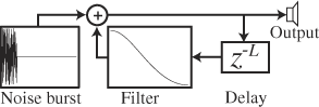 English: Schematic for Karplus-Strong algorithm.
 Filter
 Filter Bass Drum of Awesome
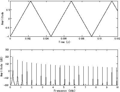 A bandlimited triangle wave pictured in the time d...
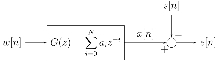 English: Diagram of a finite impulse response Wien...