Magnatism & the Things We THINK We Know About It!
By Austin D. Ritchie
Magnatism is a wonderous natural phenomanon. Since days before scientific
discoveries were even written down the world has been playing with the theories of
magnatism. In these three labs we delt with some of the same ideas which have pondered
over for long before any of us were around. In these conclusions we will take a look at
these ideas and find out what exactly we have learned.
To understand the results of the lab we must first go over the facts about
magnatism on the atomic level that we have discovered. The way magnatism works is
this: magnatism is all based on the simple principle of electrons and there behavior.
Electrons move around the atom in a specific path. As they do this they are also rotating
on there own axis. This movement causes an attraction or repultion from the electrons
that are unpaird.
 Simulation of the interaction between Earth's magn...
 This image was selected as a picture of the week o...
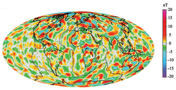 English: Lithospheric Magnetic Anomalies. A modele...
They are moving in two directions though causing a negative and
positive charge. In the case of magnatism though we find that these elements have a lot
of unpaired electrons, in the case of iron, Fe, there are four. What happens then in the
case of a natural magnet the unpaired electrons line up or the magnet in a specific
mannor. That is all the atoms with unpaired electrons moving in a direction which
causes a certain charge are lined up on one side and all the atoms with the opposite
charge move to the other side. The atoms then start to cancel each other out as they
approach the center of the magnet. This all happens at the currie point where these
atoms are free to move and then when cooled and the metel becomes solid the atoms can
no longer move (barely) causing a 'permanent' magnet (as in the diagram on the next
page). This same principle can be applied to a piece of metal that has been sitting next to
a magnatized piece of metel in that over the long time they are togather the very slow
moving atoms in the metal situate in the same fassion also creating a magnet. Now that
we know the basics lets begin with the experiments.
Part one of the lab started us on our journey. In this part we took an apparatus
with wire wrapped around it put a compass in the middle of the wire wraps. The setup
was arranged so that the wraps were running parralel with the magnetic field of the earth,
that is they were north-south. With this setup we were able to force a current through the
coils of the apparatus by means of a 6V battery and this created a magnetic field. This is
because the movement of electrons (which electrisity is) causes the presents of a
magnetic field. Now that we know we have a magnetic field running around the compass
we cbegan the experiment. What we did was take the magnetic field of the coils
begining with one coil and continued until we had five. What we learned from this is
that with every extra coil we placed around the compass the motion that the interaction of
the two magnetic fields caused increased. These magnetic feilds being the earth's and the
coils. What this means is that not only does electicity create a magnetic field but that
there is a direct relationship between the amount of current and the strength of the
magnetic field it creates. This leads us to the relationship: Bc õ I and then by figuring
in the constant we find that we can derive our first equation Bc = k I. This can also be
supported by the data we collected in the lab when we see that as the measured currents
went up the amount of motion went up which mathmaticly indicates that the magnetic
field strength went up.
But we don't only find this equation but we also find that as the current (or more
so the magnetic field it creates) acts upon the initial magnetic field of the earth we get the
motion in the compass. This leads us to the first part of our left hand rule. The left hand
rule for a straight conductor says that when the lines of flux are created they repel from
the north end of the compass in a certain direction (depending on which way the charge
is moving). This can be explained by our experiment's data in part one also because as
we introduced the current to the earth's magnetic field we found that it created the motion
on the compass. This all agrees with the left hand rule.
Lastly, we found in this part of the lab that magnetic field, represented by B, is a
vector. We can say this because we know that a vector is anything that has both a
magnatude and a direction. Now we need to prove that B has these features. This can be
done by looking back on our lab and remembering that as we found the value for B it was
the strength of the magnetic field. Now strength indicates that there is a magnatude to
the field, thus giving us the first part of a vector. To finalize the theory we look back at
the lab and find that as we changed the flow of the electrons in the coils the motion on
the compass changed also. What this tells us is that the magnetic field of the current
passing through the wire has a direction to it also. Knowing this we can deduce that B is
infact a vector. A second, less definite, manor to find that B is a vector is to recall that in
the equation B = k I we have one definite vector in the I (from earlier labs) and since we
know that you much have a vector on each side of the equation in order for it to balance
out and we know that k is a constant (therefore not a vector) the only possiblility is that B
is infact a vector.
In addition to these 'required' conclusions we also found, as stated earlier, that
when you have current you also have a magnetic field. This is important because it gives
us another means in which to create magnetic fields other than the use of 'natural'
magnets. But to put this theory into mathmatical application we can use the formula of
Fb = B I L and say that since we know it takes two magnetic fields to cause motion
(represented in this equation by F) and we know that B is in itself a magnectic field we
can deduce that the value for 'I L' is infact the value for and thus equivilant to a second
magnetic field.
The next lab we conducted consisted of a factory made coil, an ammeter to find
the value of the current we were creating and a bar magnet to act as a magnetic field.
What we did was thrust the bar magnet N end first through one of the sides of the coil
and found that this created a current. This happened because what we were actually
doing was taking one magnetic field and putting it to motion thus creating antother
magnetic field, which in this case happened to be an electical current. This experiment
once agains deals with, obeys and exemplifies the left hand rule, but this time for a
celenoid. What that means is that as we were thrusting the magnets N end into the coil
we induced a positive amount of current simply because of the direction in which the
LHR tells us that the current should go. Now the converse is also true in this case. What
that means is that when you either thrust the N end of the magnet out of the coil or thrust
the S end into the coil we find that a negative amount of current is invoked.
Our next conclusion has to deal with a combonation of theories being Lenz's law
and induction. Now we know from above that as we thrust the N end of the magnet into
the coil we achieved a positive current and with a S end a negative current what this
shows us is that there is conservation of energy here. Conservation of energy is a main
part of Lenz's law. The reason we can say that this is conservation of energy is because
when a charge was induced it is the opposite (pos/neg) of the the current that it was
induced by. We can further Lenz's law by remembering that the faster we thrust the
magnet into the coil the more current that was produced. This also shows us the
principle of conservation of energy because the more energy put into the system the more
current we got back out. This theory can be easily concluded by saying that only when
you have perpendicular motion of a magentic field can a current be produced. All these
currents and fields are created by what is called induction. What this means is that we
are not actually touching the physical objects togather (contact) but instead just placing
them near each other so that their magnetic fields are 'touching' and the motion or force
can result.
That moves us onto the last part of the lab where we used the same coil from part
two and hooked it up in a system (pictured on next page) where we could measure the
current strength and have our teeter-totter with an electric current running through it
within the lines of the magnetic field of the coil. What we are able to do with this setup is
run a current through the system creating a pair of magnetic fields on the coil and the
loop (on the end of the teeter-totter). The diagram below shows the setup that was used
along with a vector diagram. What this tells us is that the force, Fb or magnetic force, on
the end of the TT that is inside the coil is infact a vector. Once again that means that it
has both magnatude and direction. Now we learned last term that force is always a
verctor and therefore can assume that this too is a vector but there is even more evidence
to support this. You see the force that is acting upon the end of the TT that is outside the
coil is being acted on by the force of gravity. This gravitational force, Fg on the diagram,
has the value Fb * m, where 'm' is the mass of the object that is setting on the end of the
TT. Since we know that gravitational force is a vector and we see that the TT is balanced
out we know that the forces acting upon both sides of the TT must be equal, otherwise
one side would be lowered like in the next diagram (b). Here, in b, we see the TT before
the current, and therefore the magnetic fields acting on eachother causing magnetic force,
has been introduced to the system. As we see the TT is now unballanced. Now look
back at the first diagram and notice that the vectors of Fb and the value of Fg * m are
equal. Since we massed the 'weight' we used to uniformity and we know that
gravitational force is 9.8 m/s2 we then know the value of Fb as well as the fact Fb is
indeed a vector that is ofsetting the gravitational force vector. We know this because if
Fb was not a vector the TT would never balance. We also notice that mathmatically
there is a relationship. That is that the units for the value of Fb are kg*m/s2 which we
know to be velocity and therefore a vector as velocity is.
This leads us to the first of three very important equations. This equation,
Fb = Bc * I * Lloop
then gives us the experimental value for Bc which is important because this could not be
measured directly in our lab. We find this value now very useful because it does not
depend on any of the factory specifications for the coil which we prove to not be true
later. This is the most important equation in this section of the lab for that very reason.
This is because now that we know the experimental value of Bc without using the factory
specs we can use that value in the next two equatins to find experimental values for the
factory constants and therefore prove those set values right or wrong.
The next equation,
Bc = k * Ic * Iloop * Lloop
now serves two purposes. One, it allows us to calculate a 'factory' value for the
magnetic field, knowing the length of the loop (L), the current through the loop and coil
(I) and the constant (k) from the factory. We do this so that we can compare this value to
our experimental value for Bc and see how close they are. Two, is that you can plug in
the experimental value for Bc and the two I's and the L and find a value for 'k' based on
our data. We then compared the two numbers of each to find that in actuallity the factory
and the experiment disagree, but minorly. This could be due to either error on our part or
on the factories but at least lets us know that we are relatively close.
Lastly, we look at the equation,
Bc = u * N * I / L
which does the same basic thing as the previous one does accept in this one we can plug
in all numbers but the number of turns (N) and then solve for the experimental number of
turns. Or we can plug in the factory number of turns and all the rest accept Bc and solve
for that leaving us with another factory value for Bc. Once again we compare these
numbers to the numbers we had previosly and this time we find that the number of turns
on the coil is experimentally less to a great extent and that Bc for this equation is
extreemely different than the ones solved for above. What this told us was that while the
factory value for 'k' was relatively close the factory set number of turns is actaully way
off.
All this leads us to the way that the Earth's magnetic field works. We have used
this field in the lab but not defined it. But through our experiment we can make some
conclusions. What we learned combined with the diagrams and researched data that we
acquired shows us that the earth does not have a bar magnet in the middle of it that is
making it attract and repel things like compasses but rather that their is something else
going on. After searching and thinking hard we found that the earth actually has no
magnetic field in it's center but rather that the magnetic pull we feel comes from the
friction (friction induces a current, earlier labs) of the outter layer of molten earth and the
top layer of its' crust and the current then creating a magnetic field as we know occurs.
We can say that there is no charge in the middle because we know that the center of the
earth is extreemly hot and with that it must be above the currie point, where a magnet's
electrons situate and create, when cooled, a magnet. What this means is that it's too hot
for a magnet to possibly exhist at that temperature. We also know that there is no magnet
there because of the simple fact that on the atomic level a magnet cannot exist in a liquid
because of the uniformity a strong magnet requires and the 'loosness' of the molecules in
a liquid, that is how free they are to move. Now since we know that the center of the
earth is molten, a liquid, and therefore a magnet cannot exist there. But this doesn't
explain all of what we have learned. We also see that the magnetic 'poles' of the earth
are actually not as we think of them. As the next diagram shows the earths poles are
actually made up of a magnetic north and south pole and a geological north and south
pole. But these poles very. The magnetic poles are actually slightly off center to the
geological poles. Along with this we can say that because of the scientists of the past we
actually call the magnetic south pole the north pole and vise-versa. This isn't due to some
phenomanon but rather the fact that when we think of the north pole we think of the
earth's pole that the north end of a compas (or any magnet) is attracted to. This is
actually the south end of the earths magnetic field, explaining this confusion.
All of this was learned on our very difficult trip through the world of the magnet
and now that we have conducted these experiments, done the research, and made these
conclutions we now know that much more about the voo-doo world of the magnet!